Beyond the baseline: addressing tail risk in Expected Credit Loss models

A follow-up to our previous analysis

In our previous article – Navigating the new trade war: implications on Expected Credit losses  – we explored the rise in provisioning needs triggered by both direct impacts (sector/geography-specific exposure to tariffs) and indirect impacts (macroeconomic degradation influencing model parameters). Through simulations and stress testing, we showed how seemingly modest shocks could drive significant increases in Expected Credit Losses (ECL), particularly through the nonlinear dynamics of IFRS 9 frameworks.

We concluded with a call to widen the risk horizon – to challenge assumptions, revisit scenarios and account for “unknown unknowns” in an increasingly volatile global economy.

Are we stressing enough?

As institutions continue refining their risk models, an important question emerges: How do we know if our downside scenarios are sufficient? In particular, is the stress we are applying severe enough to capture the potential nonlinear behaviour of credit losses?

Regulators and auditors often require the use of “severe but plausible” scenarios. But in periods of heightened uncertainty, relying solely on baseline and modest downside paths may not capture the full risk picture, especially when models are convex in nature.

Introducing convexity in credit risk

Convexity refers to a relationship where the output increases at an accelerating rate relative to the input. In credit modelling, this means that credit losses do not rise linearly with deteriorating macroeconomic conditions: they can grow disproportionately as the environment worsens. This nonlinearity highlights the importance of ensuring that downside scenarios are sufficiently wide-ranging to capture such effects, particularly when small shifts in key variables can lead to much larger increases in expected losses.

To illustrate this, consider a naïve ECL model with a single loan, with an Exposure At Default (EAD) of 100 USD, a Loss Given Default (LGD) of 50%, and the following Probability of Default (PD) model:

In this case, we know that a quadratic equation such as the one denoted above is convex. Given that we fixed the LGD and EAD with constant value, the ECL function (ECL = PD x LGD x EAD) will take the same characteristics as the PD function.

Using the above information, we can illustrate the resulting ECL as follows:

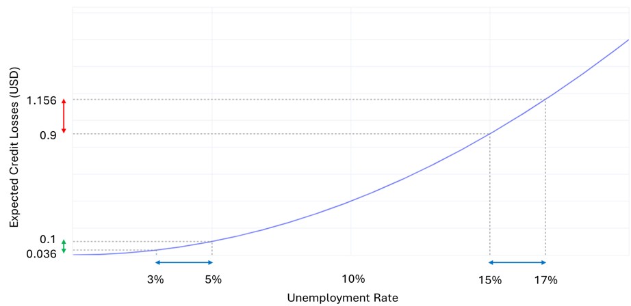
In the graph, we have highlighted three comparisons using arrows. The blue arrows along the x-axis represent two identical increases in unemployment, each spanning a 2% change. However, the green and red arrows along the y-axis show that the resulting change in ECL is not the same. The green arrow, corresponding to the increase in ECL between 3% and 5% unemployment, is significantly smaller than the red arrow, which represents the increase in unemployment between 15% and 17%.

This difference illustrates the effect of convexity: for a constant change in the input variable (in this case, unemployment), the output (ECL) increases more sharply at higher levels of stress. This behaviour is highly relevant in today’s macroeconomic environment.

As unemployment rises, the risk of credit deterioration tends to escalate faster due to compounding pressures: declining consumer demand, tighter credit conditions, and broader financial stress. In such contexts, assuming a linear relationship between macroeconomic variables and credit losses could severely underestimate tail risks. This example reinforces why downside scenarios must be tested across a broad range of economic conditions, not just to meet regulatory expectations, but to better prepare for nonlinear, adverse outcomes that may materialise when volatility increases.

Are your risk models underestimating stress?

Now that we understand that ECL functions can behave nonlinearly in response to macroeconomic inputs, the next question becomes: how can we test whether our models are actually convex?

In our earlier example, we worked with a highly simplified, one-dimensional ECL model; a single loan with fixed EAD and LGD, and a quadratic PD function. While useful for illustration, real-world IFRS 9 models are significantly more complex, combining multiple risk drivers and variables. Convexity is not necessarily evident.

One way to explore convexity more formally is through the lens of Jensen’s inequality. This inequality is a principle in mathematics that provides a practical and elegant test for convexity. While abstract in theory, it offers a surprisingly effective diagnostic for risk models.

Formally, based on Jensen’s inequality, a function is convex if and only if:

In simple terms: if a function is convex, the expected value of the function is greater than or equal to the function of the expected value. Translating this into credit modelling: if your ECL model is convex, the ECL calculated using an average macroeconomic input (e.g., average unemployment across scenarios) will be lower than the average ECLs calculated for each scenario individually.

While this relationship can easily be demonstrated through numerical examples, we have not included them here in order to keep the focus on the conceptual implications for risk practitioners.

From concept to application: using convexity to assess tail risk

“Convexity does not change your models – it changes how you read them.”

Convexity is not a “pass or fail” condition for risk models. Instead, it serves as a powerful tool to help institutions determine whether their risk frameworks are sufficiently capturing tail risk – particularly in a world where stress can emerge quickly and from multiple directions.

In the context of the ongoing trade war and broader geopolitical uncertainty, macroeconomic conditions can deteriorate in ways that are both nonlinear and asymmetric. As shown in our earlier analysis, tariffs can trigger direct shocks to specific sectors and ripple effects through macroeconomic variables like inflation, GDP, and unemployment. These effects can compound, making traditional scenario structures – centred around a base case and a modest downside – potentially insufficient.

This is where convexity comes in. If ECL models display convex behaviour, they signal that small increases in stress variables may result in disproportionately higher losses. In such cases, institutions might already be capturing tail risk through multiple scenarios. But when convexity is absent, or weak, it may indicate that:

• Scenario weights place too much emphasis on central paths;
• Tail events are not being adequately represented; or
• Additionally, more severe downside scenarios are needed to reflect the full distribution of plausible risks.
• In linear models, downside and upside effects may offset each other, masking the true impact of tail events.

Importantly, this does not mean the model is wrong, only that its outputs need to be interpreted with care, especially when used for provisioning, overlay justification, or regulatory and audit discussions.

In the face of mounting economic complexity, convexity testing offers institutions a simple but powerful checkpoint: are we truly capturing the shape of the risk ahead, or are we relying too heavily on linear thinking in a nonlinear world?